Comparison of Machine Learning-Based Radioisotope Identifiers for Plastic Scintillation Detector

Article information

J. Radiat. Prot. Res. 2021;46(4):204-212

Publication date (electronic) : 2021 November 27

doi : https://doi.org/10.14407/jrpr.2021.00206

Byoungil Jeon ¹, Jongyul Kim ², Yonggyun Yu ¹, Myungkook Moon^,²

¹Artificial Intelligence Application & Strategy Team, Korea Atomic Energy Research Institute, Daejeon, Korea

²Neutron Science Division, Korea Atomic Energy Research Institute, Daejeon, Korea

Corresponding author: Myungkook Moon Neutron Science Division, Korea Atomic Energy Research Institute, 111 Daedeok-daero 989beon-gil, Yuseong-gu, Daejeon 24057, Korea E-mail: moonmk@kaeri.re.kr

Received 2021 May 4; Revised 2021 June 14; Accepted 2021 June 17.

Abstract

Background:

Identification of radioisotopes for plastic scintillation detectors is challenging because their spectra have poor energy resolutions and lack photo peaks. To overcome this weakness, many researchers have conducted radioisotope identification studies using machine learning algorithms; however, the effect of data normalization on radioisotope identification has not been addressed yet. Furthermore, studies on machine learning-based radioisotope identifiers for plastic scintillation detectors are limited.

Materials and Methods:

In this study, machine learning-based radioisotope identifiers were implemented, and their performances according to data normalization methods were compared. Eight classes of radioisotopes consisting of combinations of ²²Na, ⁶⁰Co, and ¹³⁷Cs, and the background, were defined. The training set was generated by the random sampling technique based on probabilistic density functions acquired by experiments and simulations, and test set was acquired by experiments. Support vector machine (SVM), artificial neural network (ANN), and convolutional neural network (CNN) were implemented as radioisotope identifiers with six data normalization methods, and trained using the generated training set.

Results and Discussion:

The implemented identifiers were evaluated by test sets acquired by experiments with and without gain shifts to confirm the robustness of the identifiers against the gain shift effect. Among the three machine learning-based radioisotope identifiers, prediction accuracy followed the order SVM >ANN>CNN, while the training time followed the order SVM>ANN>CNN.

Conclusion:

The prediction accuracy for the combined test sets was highest with the SVM. The CNN exhibited a minimum variation in prediction accuracy for each class, even though it had the lowest prediction accuracy for the combined test sets among three identifiers. The SVM exhibited the highest prediction accuracy for the combined test sets, and its training time was the shortest among three identifiers.

Keywords: Plastic Scintillation Detector; Radioisotope Identifier; Machine Learning; Deep Learning; Data Normalization

Introduction

Radiation portal monitors (RPM) are deployed in national facilities and borders, and operated to prevent sabotage of the facilities or nuclear smugglings through the borders. These mostly use plastic scintillators that have lower costs and larger detection volumes by up to tens of liters than other types of radiation detectors [1–5]. However, RPMs based on plastic scintillators are primarily used for counting applications to determine the existence of radioactive materials, because they have poor spectroscopic capabilities owing to their poor energy resolution and the absence of a photo peak. Therefore, RPMs that need capabilities of radioisotope identification must use inorganic scintillation detectors. To overcome the difficulty of radioisotope analysis using plastic scintillation detectors, several methods for pseudo-spectroscopy have been developed based on spectral signal processing, such as the energy windowing method [6–9], energy-weighted algorithm [10, 11], and F-score method [12].

In addition, pattern recognition applications have been developed for radioisotope identification from radiation measurements. Several researchers introduced radioisotope identification based on classical pattern recognition methods, such as data matching for silicon detectors [13], data matching [13–15] and statistical data analysis [16–18] for inorganic scintillation detectors, and data matching [19, 20] for plastic scintillation detectors. Machine learning-based radioisotope identifiers have also been studied by several researchers. Studies on the quantitative analysis of radionuclides based on neural networks were introduced for silicon detectors [21, 22]. For inorganic scintillation detectors, several researchers conducted radioisotope identification using the support vector machine (SVM) [23] and variations of neural networks [24–30]. In the case of plastic scintillation detectors, artificial neural network (ANN)-based applications for radioisotope identification have been introduced [31–34].

Machine learning-based radioisotope identifiers have exhibited superior performance with measured spectra with a high level of uncertainties in various studies; however, the impact of data normalization on radioisotope identification using machine learning algorithms has not been addressed yet. Generally, data normalization for machine learning is known to make the optimization process, i.e., the model training process, faster and more accurate. Therefore, data normalization is an essential aspect of machine learning algorithms. In this study, machine learning-based radioisotope identifiers for plastic scintillators were implemented, and their performances according to data normalization methods were compared. Eight classes were defined by combining ²²Na, ⁶⁰Co, and ¹³⁷Cs, including background. The SVM, ANN, and convolutional neural network (CNN) were implemented as radioisotope identifiers with six data normalization methods, and their performances were compared.

Materials and Methods

1. Machine Learning Approaches

In this paper, each machine learning algorithm was selected for the following reasons. An SVM was selected, as it was the most powerful method for pattern recognition problems before deep learning became popular. The CNN was selected because it is a typical deep learning method. Although the performance of the CNN is well-known with regard to image data, the input data in this paper are not images, i.e., two-dimensional data, but spectra, i.e., one-dimensional data. Information extracted by a convolution operation on input data is a sort of relationship near the subset of data, so it is possible to express the changes in different parts of the data. Consequently, a convolution operation is useful for extracting features in image data, e.g., edges where the change in pixel values occurs conspicuously, in image processing. However, the input data in this paper are the spectra of plastic scintillator; they do not show significant changes owing to their poor energy resolution and the absence of a photo peak. Therefore, the CNN might not be appropriate for radioisotope identification from the spectra of plastic scintillation detector. To compare the CNN with other neural network approaches, an ANN was selected.

2. Data Set Generation

1) Experimental environment used to measure gamma spectra

To measure spectra, a polystyrene scintillation detector that has a cylindrical shape of dimensions 30×50 mm² (diameter× height) was used, and a PMT (Model R2228 and E990-501; Hamamatsu Photonics, Shizuoka, Japan) was coupled with the detector sequentially. Optical grease (Model BC630; SaintGobain, Cedex, France) was spread between the crystal and PMT for optical coupling. A signal processing module (DP5G; Amptek Inc., Bedford, MA, USA) was used as a preamp, shaping amp and an MCA, and operating voltages were supplied by a high voltage supplier (Model NHQ 224M; ISEG, Radeberg, Germany).

Gamma-ray spectra were measured in an aluminum dark box for optical shielding of the detector. The dark box consists of a 10 mm-thick aluminum layer with internal dimensions of 440×400×900 mm³ (width×height×length). At the door of the box, 1 mm-thick rubber layer was attached for optical shielding. Fig. 1 shows the dark box and experimental setup.

Fig. 1.

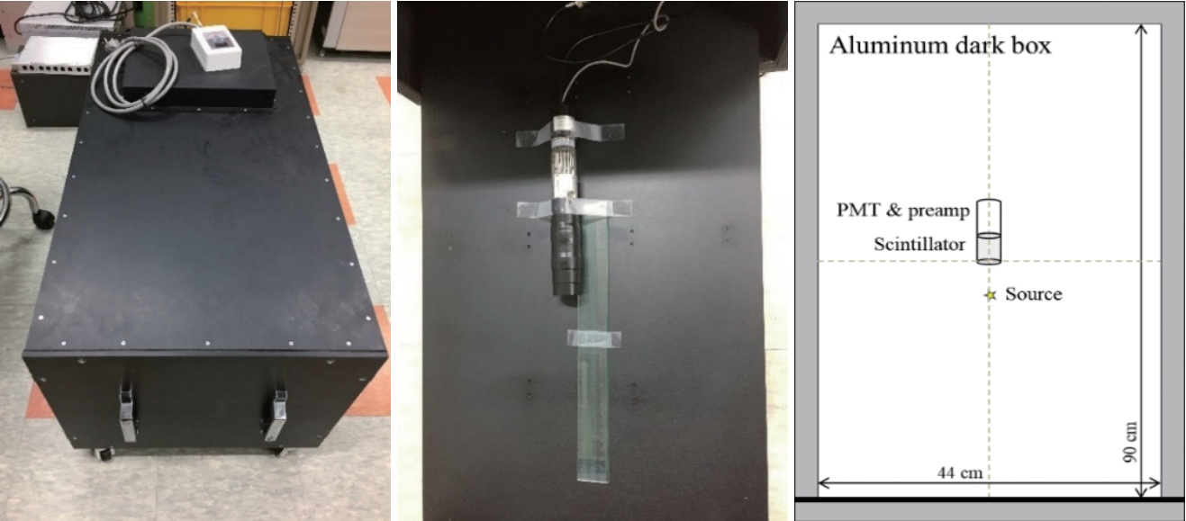
Aluminum dark box and experimental setup. PMT, photomultiplier tube.

²²Na, ⁶⁰Co, and ¹³⁷Cs were utilized as the gamma-ray sources. The gamma-ray sources were selected because of following reasons: ⁶⁰Co and ¹³⁷Cs were selected because they are the typical gamma-ray sources. Owing to the poor energy resolution of plastic scintillators, it is challenging to distinguish between a combination of radiation sources that emit gamma-rays with similar energies. ²²Na emits photons that have an energy of 511 keV, which is similar to the energy of photons emitted by ¹³⁷Cs, and 1,274 keV, which is similar to the energy of the photons emitted by ⁶⁰Co. To confirm the identification performance for combinations that are not easily distinguishable from spectra with poor energy resolutions (e.g., ¹³⁷Cs & ⁶⁰Co from ²²Na & ⁶⁰Co), ²²Na was selected as an additional gamma-ray source. Table 1 shows a summary of classes for identification of radioisotopes.

Table 1.

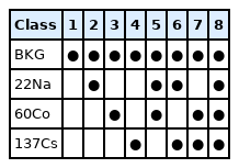
Definition of Classes for the Radioisotope Identification Problem

To measure the spectra, the window of a detector was placed at the center of floor of the dark box. Owing to the different half-lives of each gamma emitter, the distances from the window of the detector to a source were adjusted until the number of counts was similar. By numerous trials, the distances were decided as 3 cm for ²²Na, 5 cm for ⁶⁰Co, and 7.5 cm for ¹³⁷Cs.

2) Monte Carlo simulations

MCNP version 6.2 [35] was utilized for the Monte Carlo simulation. The experimental environment was implemented in the simulation code. The compositions of materials were defined by referring to a report [36], and the densities of the materials were 2.6898 g/cm³ for aluminum layer, 1.2 g/cm³ for rubber layer, and 1.06 g/cm³ for polystyrene scintillator. Each source was defined as a point source, the cutoff energy was set to 1 keV, and the history number was set to 108. The Gaussian energy broadening parameters for Monte Carlo simulations were calculated by a parametric optimization technique [37] and were set as follows: “a” is 0.0258, “b” is 0.212, and “c” is 1.8678.

3) Dataset generation

In this study, we approached the identification of radioisotopes as a classification problem, and each application was trained by supervised learning. The training and test sets were generated as follows. The test set was derived from the experimental results. In the experimental environment explained in Materials and Methods section (2.1 Experimental environment), the spectra for each class were measured 100 times for 10 seconds. The measured spectra had 512 channels, but counts from 1 to 10 channels were ignored because of the setting for low level discrimination.

The training set was generated by a random sampling technique. The measured and simulated probabilistic density functions (PDFs) were utilized to generate the training set. The PDFs were calculated as follows: in the experimental setup explained in Materials and Methods section (2.1 Experimental environment), the spectra for each class were measured for 30 minutes to obtain the fine spectra. For the fine spectra, each fine spectrum was normalized by dividing the integral value of each spectrum. In this manner, the measured PDFs of the counts for each energy bin were calculated for each class. By the Monte Carlo simulation explained in Materials and Methods section (2.2 Monte Carlo simulations), the spectra for each class were simulated. Channel to energy calibration was conducted by a parametric optimization technique [37]. As it is difficult to simulate realistic background spectra, the measured background spectrum was added to the simulated spectra for all classes. Then, simulated PDFs were also calculated analogously with the calculation of measured PDFs.

Using the calculated PDFs, the training set was generated as follows: (1) the number of sampling counts varied between 200 and 500 for the background class and between 1,000 and 3,000 for other classes. These ranges were set by considering the total counts of each class in test set; (2) spectral data was randomly sampled based on the calculated PDFs up to the decided number of sampling counts; (3) the spectral data of 450 channels were extracted from the original spectra of 512 channels to enhance robustness against peak or gain shift effects. The initial channel for spectra extraction was randomly selected in a range of 11 to 30. In total, 500 spectra for each class (totally 4,000 for all classes) were sampled by the training set generation mentioned above and used as the training set for the machine learning algorithms. For each case, the training set consisted of 50% sampled data based on the measured PDFs and 50% based on simulated PDFs. Fig. 2 shows an example of a procedure for generating the training set. We applied six data normalization methods to the generated training set and acquired test set. Applied methods are summarized in Table 2.

Fig. 2.

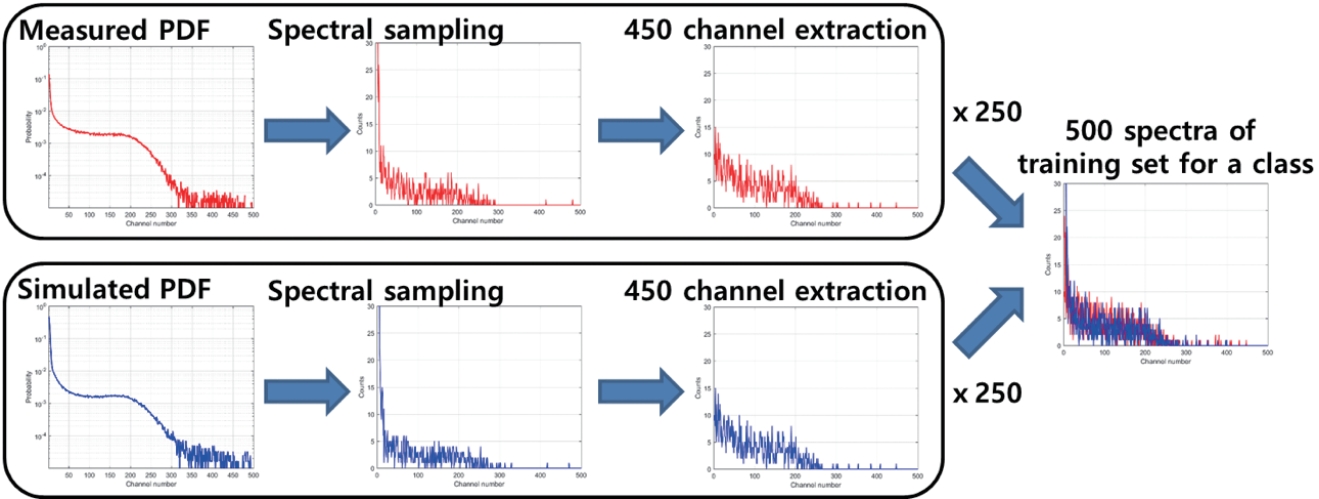
Example of a procedure for generating a training set for a class of ⁶⁰Co. PDF, probabilistic density function.

Table 2.

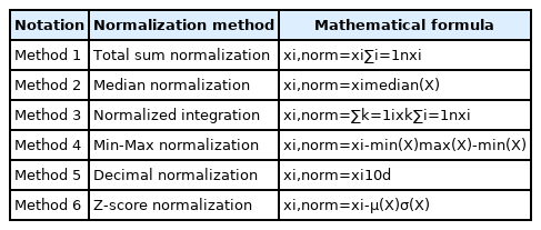
Summary of the Data Normalization Methods

In this paper, an additional dataset for validation was not generated, but a cross-validation technique was used to validate the training results. In the cross-validation, the subset was extracted from the training set and used for validation. The validation fraction was set to 0.2, which indicates that 20% of the training set was extracted for validation. For the SVM, a five-fold cross-validation was used, which indicates that cross-validation was repeated five times with different subsets, and averaged result was output as the final validation result. For the ANN and CNN, the subset for validation was extracted, and cross-validation was conducted for every epoch.

3. Model Implementation

SVM was implemented in a Python environment with the LIBSVM library [38], and tunable parameters were found by the grid search method that was provided as a function of the library. ANN and CNN were implemented in the Python environment library using the TensorFlow library [39]. The tunable hyper-parameters for ANN were defined as follows: the number of layers, number of neurons for each layer, dropout rate, learning rate, and batch size. Tunable hyper-parameters were defined to be analogous to those of an ANN, but several parameters were added: the number of convolution layers and size of the convolutional kernel. The hyper-parameters of the ANN and CNN were found by the Bayesian optimization technique [40]. A cross-entropy function was used as a loss function, and the Adam optimizer was used for training ANN and CNN models. The rectified linear units (ReLU) function was used as an activation function of hidden layers, and the softmax function was used as an activation function of the output layer. The maximum epochs used to train a model were set as 1,000. Furthermore, the early stopping option was applied to prevent overfitting issues. The monitoring value for early stopping was set as validation accuracy, and the patience epoch number was set to 50.

Results and Discussion

1. Identification Results

The training set and test set were normalized by methods 0 to 6. For here, method 0 denotes raw data, i.e., data without normalization, and the others are listed in Table 2. The implemented SVM, ANN, and CNN were trained and tested using training sets and test sets normalized by each method. Hyper-parameter tunings were conducted for each normalization method. Fig. 3 shows the averaged accuracy of the SVM, ANN, and CNN according to the data normalization methods. As shown in Fig. 3, SVM and ANN exhibit the highest identification accuracy with method 5, i.e., decimal normalization, and the CNN has the highest accuracy without data normalization.

Fig. 3.

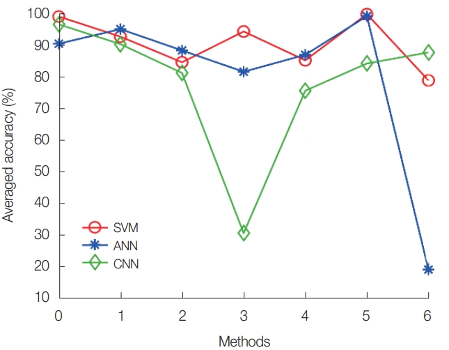
Averaged prediction accuracy of support vector machine (SVM), artificial neural network (ANN), and convolutional neural network (CNN) according to data normalization methods.

2. Gain Shift Sensitivity

Spectra measured by plastic scintillation detectors can cause gain shift effects owing to the calibration drift or temperature effect. To obtain robust machine learning models for radioisotope identification against gain shift effects, we added 450 channel extraction processes during the training set generation procedure as described in Materials and Methods section (2.3 Dataset generation). To confirm that our models have robustness against the gain shift effect through the channel extraction process, we applied the gain shift effect by adjusting the gain value of the linear amplifier in the positive and negative directions. The magnitude of the gain shift were ±10% of the energy bins for the positive and negative directions.

We conducted radioisotope identification for the test set with gain shift effects using the pre-trained SVM, ANN, and CNN. Fig. 4 shows the averaged prediction accuracy of the SVM, ANN, and CNN according to the data normalization methods for the test set with positive and negative gain shifts. As shown in Fig. 4, the best data normalization methods for the SVM, ANN, and CNN were different depending on the gain shift effects. For a positive gain shift, the SVM had the highest accuracy with method 3, i.e., normalized integration, and the ANN and CNN had the highest accuracies with method 1, i.e., the total sum normalization. For the negative gain shift, the SVM had the highest accuracy with method 3, i.e., normalized integration, the ANN had the highest accuracy with method 1, i.e., total sum normalization, and the CNN had the highest accuracy without data normalization.

Fig. 4.

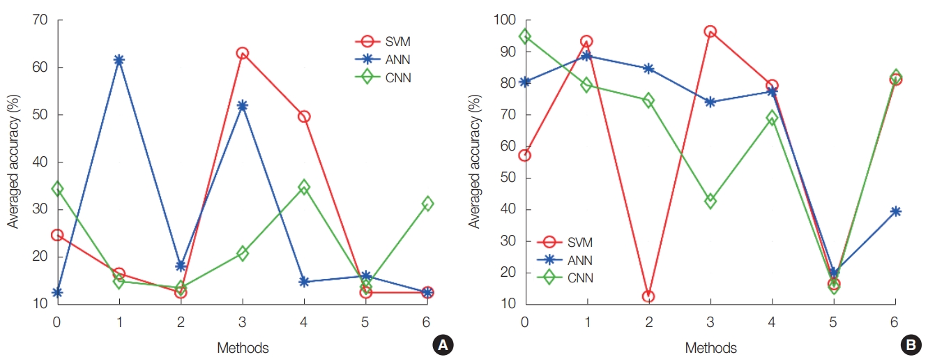
Averaged prediction accuracy of the support vector machine (SVM), artificial neural network (ANN), and convolutional neural network (CNN) according to data normalization methods for the test set with gain shifts in (A) positive and (B) negative directions.

3. Gain Shift Sensitivity Combined Results on Test Sets with and without Gain Shift Effect

To select the best normalization methods for the SVM, ANN, and CNN, we confirmed the averaged prediction accuracy for the test sets with and without the gain shift. Fig. 5 shows the prediction accuracy for combined test sets with and without gain shift effects in the SVM, ANN, and CNN according to the data normalization methods. Table 3 shows the determined hyper-parameters for the SVM, ANN, and CNN for the data normalization methods.

Fig. 5.

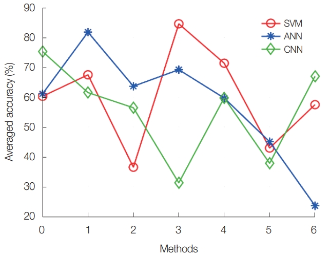
Averaged prediction accuracy for combined test sets with and without gain shift effects in the support vector machine (SVM), artificial neural network (ANN), and convolutional neural network (CNN) for different data normalization methods.

Table 3.

Determined Hyper-parameters of the SVM, ANN, and CNN for Different Data Normalization Methods

4. Discussions

Among the three machine learning-based radioisotope identifiers, prediction accuracy for combined test sets with and without gain shift increased in the order SVM>ANN>CNN. The training time increased in the order SVM>ANN>CNN. It took 2.867 seconds to train an SVM model with the best hyper-parameters described in Table 3 using a desktop that has CPU of 4 kHz Intel Core i7 and RAM of 32 GB. For training of an ANN and CNN, a graphics processing unit workstation was used, which has four units of the GeForce GTX1080Ti with 11 GB memory. Despite this, however, it took 149.089 seconds and 2270.678 seconds, respectively to train an ANN and a CNN with the best hyper-parameters described in Table 3. These training times are the time taken to train a model for each method.

The identification performances of the implemented radioisotope identifiers can be changed according to the quality of spectral data. If the identifiers are trained and tested with data that has a higher number of counts than ours, the identification performance could be enhanced. Furthermore, the ANN and CNN may have better identification performances, if they have deeper layers or advanced structure, i.e., deeper convolution layers [41, 42], residual shortcut connection [43], dense connection [44], etc. The depth of the hidden layers and structure of neural networks were associated with the number of training sets and the time to train a model. Therefore, a model with deeper hidden layers or advanced structure needs not only a larger number of training samples but also requires a longer training time than our neural network models. Although advanced neural networks that have deeper layers or complicated structures were not considered in this study because there’s possibility that their accuracies can be improved than those of our SVM, ANN, and CNN, further studies must be conducted to confirm their performance.

Even though our study was conducted with simulations and experiments, data used in this study may be out of practical measurements because of following limitations that we did not address. Firstly, our study was conducted with measurement data from a small plastic scintillation detector. In practice, most of radioisotope identification methods for plastic scintillation detectors are targeted to be applied on radiation portal monitors, whose volumes are over than several tens of liters. Furthermore, we fixed measuring period and position of gamma-ray sources, which may far away from realistic situations. Therefore, measurement from plastic scintillation detectors in field may have different characteristics from ours such as lack of counts or change in shape of Compton continuum because of geometric randomness of specimens and gamma-ray attenuation in specimens. Secondly, radiation sources used was limited. Although sources used in this study were typical gamma ray sources, major challenging issue of radioisotope identification in field applications may be distinguishing naturally occurring radioactive materials to reduce nuisance alarms of radiation portal monitors or special nuclear materials to prevent smugglings that may cause nuclear threats. Thirdly, the magnitude of gain shift could be higher than 10% which we set to. Therefore, further studies on these limitations are necessary to develop machine leaning based radioisotope identifiers for field applications.

Conclusion

We implemented machine learning-based radioisotope identifiers for plastic scintillation detector, and the impact of data normalization for each identifier was compared. SVM-, ANN-, and CNN-based identifiers were trained by a training set that was generated using measured and simulated PDFs, and evaluated by real measurement data. To compare the impact of data normalization on machine learning-based identifiers, we applied six data normalization methods, as well as a no normalization case, to the training set and test sets for the identifiers. The applied normalization methods are the total sum normalization, median normalization, normalized integration, min-max normalization, decimal normalization, and Z-score normalization. To build radioisotope identification models that have robustness against gain shift effects, we added a 450-channel extraction process in the training set generation procedure. For combined test sets with and without gain shift effects, the SVM had the best prediction performance with normalized integration, the ANN had the best performance with total sum normalization and the CNN had the best performance without data normalization. The prediction accuracy for the combined test sets was highest with the SVM. The CNN exhibited a minimum variation in prediction accuracy for each class, even though it had the lowest prediction accuracy for the combined test sets among three identifiers. The SVM exhibited the highest prediction accuracy for the combined test sets, and its training time was the shortest among three identifiers.

Notes

Conflict of Interest

No potential conflict of interest relevant to this article was reported.

Author Contribution

Conceptualization: Jeon B, Kim J. Data curation: Jeon B, Kim J. Formal analysis: Jeon B, Kim J. Funding acquisition: Yu Y, Moon M. Methodology: Jeon B. Project administration: Moon M. Visualization: Jeon B. Writing - original draft: Jeon B. Writing - review & editing: Jeon B, Yu Y, Moon M. Investigation: Jeon B, Kim J. Resources: Moon M. Software: Jeon B. Supervision: Yu Y, Moon M. Validation: Kim J.

Acknowledgements

This work was supported by the Korea Atomic Energy Research Institute (No. 79501-19), Ministry of Oceans and Fisheries (KIMST) (No. 20200611).

References

1. Stromswold DC, Darkoch JW, Ely JH, Hansen RR, Kouzes RT, Milbrath BD, et al. Field tests of a NaI(Tl)-based vehicle portal monitor at border crossings. In : Proceedings of IEEE Symposium Conference Record Nuclear Science; 2004 Oct 16–22; Rome, Italy. 196–200.

2. Kouzes RT, Siciliano ER. The response of radiation portal monitors to medical radionuclides at border crossings. Radiat Meas 2006;41(5):499–512.

3. Ludlum Measurements Inc. Radiation portal monitors (Model 4525 Series) [Internet] Sweetwater, TX: Ludlum Measurements Inc. c2021 [cited 2021 Aug 28]. Available from: https://ludlums.com/products/all-products/product/model-4525-series.

4. Thermo Fisher Scientific Inc. Radiation portal monitors [Internet] Waltham, MA: Thermo Fisher Scientific Inc. c2021 [cited 2021 Aug 28]. Available from: https://www.thermofisher.com/order/catalog/product/4254982?SID=srch-srp-4254982.

5. Pacific Northwest National Laboratory. Radiation detectors at U.S. ports of entry now operate more effectively, efficiently [Internet] Richland, WA: Pacific Northwest National Laboratory; 2016. [cited 2021 Aug 29]. Available from: https://www.pnnl.gov/news/release.aspx?id=4245.

6. Anderson KK, Jarman KD, Mann ML, Pfund DM, Runkle RC. Discriminating nuclear threats from benign sources in gammaray spectra using a spectral comparison ratio method. J Radioanal Nucl Chem 2008;276(3):713–718.

7. Ely J, Kouzes R, Schweppe J, Siciliano E, Strachan D, Weier D. The use of energy windowing to discriminate SNM from NORM in radiation portal monitors. Nucl Instrum Methods Phys Res A 2006;560(2):373–387.

8. Hevener R, Yim MS, Baird K. Investigation of energy windowing algorithms for effective cargo screening with radiation portal monitors. Radiat Meas 2013;58:113–120.

9. Siciliano ER, Ely JH, Kouzes RT, Milbrath BD, Schweppe JE, Stromswold DC. Comparison of PVT and NaI(Tl) scintillators for vehicle portal monitor applications. Nucl Instrum Methods Phys Res A 2005;550(3):647–674.

10. Shin WG, Lee HC, Choi CI, Park CS, Kim HS, Min CH. A Monte Carlo study of an energy-weighted algorithm for radionuclide analysis with a plastic scintillation detector. Appl Radiat Isot 2015;101:53–59.

11. Lee HC, Shin WG, Park HJ, Yoo DH, Choi CI, Park CS, et al. Validation of energy-weighted algorithm for radiation portal monitor using plastic scintillator. Appl Radiat Isot 2016;107:160–164.

12. Paff MG, Di Fulvio A, Clarke SD, Pozzi SA. Radionuclide identification algorithm for organic scintillator-based radiation portal monitor. Nucl Instrum Methods Phys Res A 2017;849:41–48.

13. Russ WR. Library correlation nuclide identification algorithm. Nucl Instrum Methods Phys Res A 2007;579(1):):288–291.

14. Min E, Ko M, Lee H, Kim Y, Joung J, Joo SK, et al. Identification of radionuclides for the spectroscopic radiation portal monitor for pedestrian screening under a low signal-to-noise ratio condition. Nucl Instrum Methods Phys Res A 2014;758:62–68.

15. Hague EJ, Kamuda M, Ford WP, Moore ET, Turk J. A comparison of adaptive and template matching techniques for radio-isotope identification In : Algorithms, technologies, and applications for multispectral and hyperspectral imagery XXV. Bellingham, WA. International Society for Optics and Photonics. 2019.

16. Runkle RC, Tardiff MF, Anderson KK, Carlson DK, Smith LE. Analysis of spectroscopic radiation portal monitor data using principal components analysis. IEEE Trans Nucl Sci 2006;53(3):1418–1423.

17. Boardman D, Flynn A. A gamma-ray identification algorithm based on Fisher linear discriminant analysis. IEEE Trans Nucl Sci 2012;60(1):270–277.

18. Sullivan CJ, Stinnett J. Validation of a Bayesian-based isotope identification algorithm. Nucl Instrum Methods Phys Res A 2015;784:298–305.

19. Ruch ML, Paff M, Sagadevan A, Clarke SD, Pozzi SA. Radionuclide identification by an EJ309 organic scintillator-based pedestrian radiation portal monitor using a least squares algorithm. In : Proceedings of the 55th Annual Meeting of Nuclear Materials Management; 2014 Jul 20–24; Atlanta, GA. 22–24.

20. Kim Y, Kim M, Lim KT, Kim J, Cho G. Inverse calibration matrix algorithm for radiation detection portal monitors. Radiat Phys Chem 2019;155:127–132.

21. Medhat ME. Artificial intelligence methods applied for quantitative analysis of natural radioactive sources. Ann Nucl Energy 2012;45:73–79.

22. Sheinfeld M, Levinson S, Orion I. Highly accurate prediction of specific activity using deep learning. Appl Radiat Isot 2017;130:115–120.

23. Hata H, Yokoyama K, Ishimori Y, Ohara Y, Tanaka Y, Sugitsue N. Application of support vector machine to rapid classification of uranium waste drums using low-resolution γ-ray spectra. Appl Radiat Isot 2015;104:143–146.

24. Abdel-Aal RE, Al-Haddad MN. Determination of radioisotopes in gamma-ray spectroscopy using abductive machine learning. Nucl Instrum Methods Phys Res A 1997;391(2):275–288.

25. Bobin C, Bichler O, Lourenco V, Thiam C, Thevenin M. Real-time radionuclide identification in γ-emitter mixtures based on spiking neural network. Appl Radiat Isot 2016;109:405–409.

26. Kamuda M, Stinnett J, Sullivan CJ. Automated isotope identification algorithm using artificial neural networks. IEEE Trans Nucl Sci 2017;64(7):1858–1864.

27. He J, Tang X, Gong P, Wang P, Wen L, Huang X, et al. Rapid radionuclide identification algorithm based on the discrete cosine transform and BP neural network. Annals of Nuclear Energy 2018;112:1–8.

28. Kamuda M, Sullivan CJ. An automated isotope identification and quantification algorithm for isotope mixtures in low-resolution gamma-ray spectra. Radiat Phys Chem 2019;155:281–286.

29. Murray SJ, Schmitz J, Balkir S, Hoffman MW. A low complexity radioisotope identification system using an integrated multichannel analyzer and embedded neural network. In : Proceedings of 2019 IEEE International Symposium on Circuits and Systems (ISCAS); 2019 May 26–29; Sapporo, Japan. 1–5.

30. Kamuda M, Zhao J, Huff K. A comparison of machine learning methods for automated gamma-ray spectroscopy. Nucl Instrum Methods Phys Res A 2020;954:161385.

31. Kangas LJ, Keller PE, Siciliano ER, Kouzes RT, Ely JH. The use of artificial neural networks in PVT-based radiation portal monitors. Nucl Instrum Methods Phys Res A 2008;587(2–3):398–412.

32. Kim J, Park K, Cho G. Multi-radioisotope identification algorithm using an artificial neural network for plastic gamma spectra. Appl Radiat Isot 2019;147:83–90.

33. Jeon B, Lee Y, Moon M, Kim J, Cho G. Reconstruction of Compton edges in plastic gamma spectra using deep autoencoder. Sensors (Basel) 2020;20(10):2895.

34. Jeon B, Kim J, Lee E, Moon M, Cho G. Pseudo-gamma spectroscopy based on plastic scintillation detectors using multitask learning. Sensors (Basel) 2021;21(3):684.

35. Werner CJ, Bull JS, Solomon CJ, Brown FB, McKinney GW, Rising ME, et al. MCNP version 6.2 Release notes (No. LA-UR-18-20808) Los Alamos, NM: Los Alamos National Laboratory; 2018.

36. McConn RJ, Gesh CJ, Pagh RT, Rucker RA, Williams R. Compendium of material composition data for radiation transport modeling (No. PNNL-15870) Richland, WA: Pacific Northwest National Laboratory; 2011.

37. Jeon B, Kim J, Moon M, Cho G. Parametric optimization for energy calibration and gamma response function of plastic scintillation detectors using a genetic algorithm. Nucl Instrum Methods Phys Res A 2019;930:8–14.

38. Chang CC, Lin CJ. LIBSVM: a library for support vector machines. ACM Trans Intell Syst Technol 2011;2(3):1–27.

39. Abadi M, Agarwal A, Barham P, Bervdo E, Chen Z, Citro C, et al. TensorFlow: large-scale machine learning on heterogeneous distributed systems [Internet] Ithaca, NY: arXiv.org. 2016 [cited 2021 Aug 30]. Available from: https://arxiv.org/abs/1603.04467.

40. Snoek J, Larochelle H, Adams RP. Practical Bayesian optimization of machine learning algorithms. Adv Neural Inf Process Syst 2012;25:2960–2968.

41. Simonyan K, Zisserman A. Very deep convolutional networks for large-scale image recognition. In : Proceedings of the 3rd International Conference on Learning Representations (ICLR); 2015 May 7–9; San Diego, CA.

42. Szegedy C, Liu W, Jia Y, Sermanet P, Reed S, Anguelov D, et al. Going deeper with convolutions. In : Proceedings of the IEEE conference on computer vision and pattern recognition; 2015 Jun 7–12; Boston, MA. 1–9.

43. He K, Zhang X, Ren S, Sun J. Deep residual learning for image recognition. In : Proceedings of the IEEE conference on computer vision and pattern recognition; 2016 Jun 27–30; Las Vegas, NV. 770–778.

44. Huang G, Liu Z, Van Der Maaten L, Weinberger KQ. Densely connected convolutional networks. In : Proceedings of the IEEE conference on computer vision and pattern recognition; 2017 Jul 21–26; Honolulu, HI. 2261–2269.

Article information Continued

This is an Open-Access article distributed under the terms of the Creative Commons Attribution Non-Commercial License (http://creativecommons.org/licenses/by-nc/4.0) which permits unrestricted non-commercial use, distribution, and reproduction in any medium, provided the original work is properly cited.

Class	1	2	3	4	5	6	7	8
BKG	●	●	●	●	●	●	●	●
22Na		●			●	●		●
60Co			●		●		●	●
137Cs				●		●	●	●

Notation	Normalization method	Mathematical formula
Method 1	Total sum normalization	xi,norm=xi∑i=1nxi
Method 2	Median normalization	xi,norm=ximedian(X)
Method 3	Normalized integration	xi,norm=∑k=1ixk∑i=1nxi
Method 4	Min-Max normalization	xi,norm=xi-min(X)max(X)-min(X)
Method 5	Decimal normalization	xi,norm=xi10d
Method 6	Z-score normalization	xi,norm=xi-μ(X)σ(X)

Name of the parameter		Search range	Determined value
Name of the parameter		Search range	M0	M1	M2	M3	M4	M5	M6
SVM	Cost parameter	2^-15–2¹⁵	2⁵	2⁹	2⁹	2³	2⁹	2⁹	2⁷
	Shape parameter	2^-15–2¹⁵	2^-15	2³	2^-15	2³	2^-9	2¹	2^-7
	Prediction accuracy	-	60.250	67.458	36.500	84.542	71.333	42.917	57.458
ANN	# of hidden layers	1–3	3	2	2	1	2	3	3
	# of neurons in 1^st layer	10–2,000	2,000	1,374	608	187	220	213	679
	# of neurons in 2^nd layer	10–2,000	2,000	416	1,567	0	687	834	1,377
	# of neurons in 3^rd layer	10–2,000	2,000	0	0	0	0	1,392	2,000
	Learning rate	0.00001–0.01	0.00001	0.00539	0.00018	0.00029	0.00404	0.00589	0.00001
	Dropout rate	0–0.6	0.0	0.2381	0.2191	0.0	0.04952	0.08804	0.6
	Batch size	2⁰–2⁷	2¹	2⁶	2⁵	2⁵	2⁵	2³	2⁶
	Prediction accuracy	-	61.083	81.750	63.625	69.167	59.667	45.042	23.583
CNN	# of convolution neurons (filter)	16–8,000	2,400	8,000	8,000	8,000	8,000	8,000	8,000
	Convolution kernel size	2–50	50	50	50	50	50	50	50
	# of hidden layers	1–3	3	1	1	3	1	1	1
	# of neurons in 1^st layer	10–2,000	1,571	2,000	1,293	2,000	1,473	2,000	946
	# of neurons in 2^nd layer	1–2,000	2,000	0	0	2,000	0	0	0
	# of neurons in 3^rd layer	10–2,000	1,346	0	0	1,131	0	0	0
	Learning rate	0.00001–0.01	0.00001	0.00001	0.00001	0.00001	0.00001	0.00503	0.00001
	Dropout rate	0–0.6	0.6	0.0	0.0	0.0	0.0	0.0	0.0
	Batch size	2⁰–2⁷	2¹	2⁰	2⁰	2⁰	2⁰	2⁶	2⁰
	Prediction accuracy	-	75.250	61.500	56.417	31.250	59.750	37.791	67.000